Evaluating the performance of machine learning models is a crucial step to understand how well your model is generalizing to new, unseen data. There are various evaluation metrics and techniques depending on the type of problem you’re working on (classification, regression, clustering, etc.). Here’s a general overview of how to evaluate a model’s performance:

Splitting Data: Start by splitting your dataset into two parts: a training set and a testing (or validation) set. The training set is used to train the model, and the testing set is used to evaluate its performance.
Metrics for Classification: If you’re working on a classification problem (categorizing data into classes), you can use metrics like:
- Accuracy: The proportion of correctly classified instances.
- Precision: The ratio of correctly predicted positive observations to the total predicted positives. It focuses on the accuracy of positive predictions.
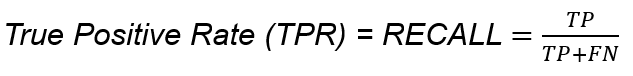
- Recall (Sensitivity or True Positive Rate): The ratio of correctly predicted positive observations to the all observations in the actual class.
- F1-Score: The weighted average of precision and recall. It balances precision and recall when they have an uneven distribution.
- Confusion Matrix: A table to describe the performance of a classification model on a set of data.
Metrics for Regression: For regression problems (predicting a continuous value), you can use metrics like:
- Mean Absolute Error (MAE): The average of the absolute differences between predictions and actual values.
- Mean Squared Error (MSE): The average of the squared differences between predictions and actual values. It gives more weight to larger errors.
- Root Mean Squared Error (RMSE): The square root of MSE, which is in the same unit as the target variable.
- R-squared (Coefficient of Determination): Indicates the proportion of the variance in the dependent variable that’s predictable from the independent variables.
Cross-Validation: To get a better estimate of your model’s performance, you can use techniques like k-fold cross-validation. This involves splitting the dataset into k subsets and training the model k times, each time using a different subset as the testing data and the rest as training data.
Hyperparameter Tuning: During evaluation, you might find that your model’s performance could be improved by adjusting its hyperparameters. Techniques like grid search or random search can help you find optimal hyperparameter values.
Overfitting and Underfitting: Keep an eye out for overfitting (model performing well on training data but poorly on test data) and underfitting (model performs poorly on both training and test data). These issues can be addressed by adjusting model complexity, using more data, or employing regularization techniques.
Domain-Specific Metrics: Depending on the domain and problem, you might need to use specific evaluation metrics. For example, in anomaly detection, you could use precision at a certain recall level.

Remember, the choice of metric depends on the specific problem you’re addressing. It’s also important to consider the business context and potential trade-offs between different metrics.

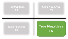
https://towardsdatascience.com/various-ways-to-evaluate-a-machine-learning-models-performance-230449055f15

TP, FP, TN, FN

https://community.sonarsource.com/t/how-to-report-a-false-positive-false-negative/37022

FP-TN-TP-TN

https://en.wikipedia.org/wiki/Sensitivity_and_specificity

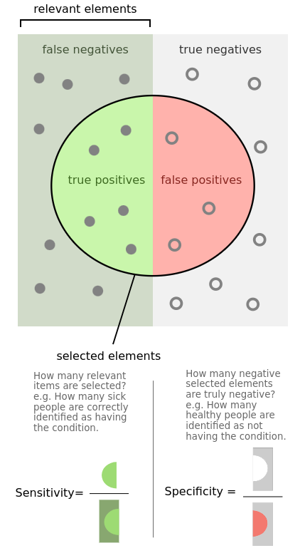
condition positive (P): the number of real positive cases in the data
condition negative (N): the number of real negative cases in the data

true positive (TP): A test result that correctly indicates the presence of a condition or characteristic
true negative (TN): A test result that correctly indicates the absence of a condition or characteristic
false positive (FP), Type I error: A test result which wrongly indicates that a particular condition or attribute is present
false negative (FN), Type II error: A test result which wrongly indicates that a particular condition or attribute is absent

sensitivity, recall, hit rate, or true positive rate (TPR): $\mathrm {TPR} ={\frac {\mathrm {TP} }{\mathrm {P} }}={\frac {\mathrm {TP} }{\mathrm {TP} +\mathrm {FN} }}=1-\mathrm {FNR}$
specificity, selectivity or true negative rate (TNR): $\mathrm {TNR} ={\frac {\mathrm {TN} }{\mathrm {N} }}={\frac {\mathrm {TN} }{\mathrm {TN} +\mathrm {FP} }}=1-\mathrm {FPR}$
precision or positive predictive value (PPV): $\mathrm {PPV} ={\frac {\mathrm {TP} }{\mathrm {TP} +\mathrm {FP} }}=1-\mathrm {FDR}$
negative predictive value (NPV): $\mathrm {NPV} ={\frac {\mathrm {TN} }{\mathrm {TN} +\mathrm {FN} }}=1-\mathrm {FOR}$
miss rate or false negative rate (FNR): $\mathrm {FNR} ={\frac {\mathrm {FN} }{\mathrm {P} }}={\frac {\mathrm {FN} }{\mathrm {FN} +\mathrm {TP} }}=1-\mathrm {TPR}$
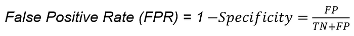
fall-out or false positive rate (FPR): $\mathrm {FPR} ={\frac {\mathrm {FP} }{\mathrm {N} }}={\frac {\mathrm {FP} }{\mathrm {FP} +\mathrm {TN} }}=1-\mathrm {TNR}$
false discovery rate (FDR): $\mathrm {FDR} ={\frac {\mathrm {FP} }{\mathrm {FP} +\mathrm {TP} }}=1-\mathrm {PPV}$
false omission rate (FOR): $\mathrm {FOR} ={\frac {\mathrm {FN} }{\mathrm {FN} +\mathrm {TN} }}=1-\mathrm {NPV}$
Positive likelihood ratio (LR+): $\mathrm {LR+} ={\frac {\mathrm {TPR} }{\mathrm {FPR} }}$
Negative likelihood ratio (LR-): $\mathrm {LR-} ={\frac {\mathrm {FNR} }{\mathrm {TNR} }}$
prevalence threshold (PT): $\mathrm {PT} ={\frac {\sqrt {\mathrm {FPR} }}{{\sqrt {\mathrm {TPR} }}+{\sqrt {\mathrm {FPR} }}}}$
threat score (TS) or critical success index (CSI): $\mathrm {TS} ={\frac {\mathrm {TP} }{\mathrm {TP} +\mathrm {FN} +\mathrm {FP} }}$

Prevalence: ${\frac {\mathrm {P} }{\mathrm {P} +\mathrm {N} }}$
accuracy (ACC): $\mathrm {ACC} ={\frac {\mathrm {TP} +\mathrm {TN} }{\mathrm {P} +\mathrm {N} }}={\frac {\mathrm {TP} +\mathrm {TN} }{\mathrm {TP} +\mathrm {TN} +\mathrm {FP} +\mathrm {FN} }}$
balanced accuracy (BA): $\mathrm {BA} ={\frac {TPR+TNR}{2}}$
F1 score: is the harmonic mean of precision and sensitivity: $\mathrm {F} _{1}=2\times {\frac {\mathrm {PPV} \times \mathrm {TPR} }{\mathrm {PPV} +\mathrm {TPR} }}={\frac {2\mathrm {TP} }{2\mathrm {TP} +\mathrm {FP} +\mathrm {FN} }}$
phi coefficient (φ or r_φ) or Matthews correlation coefficient (MCC): $\mathrm {MCC} ={\frac {\mathrm {TP} \times \mathrm {TN} -\mathrm {FP} \times \mathrm {FN} }{\sqrt {(\mathrm {TP} +\mathrm {FP} )(\mathrm {TP} +\mathrm {FN} )(\mathrm {TN} +\mathrm {FP} )(\mathrm {TN} +\mathrm {FN} )}}}$
Fowlkes–Mallows index (FM): $\mathrm {FM} ={\sqrt {{\frac {TP}{TP+FP}}\times {\frac {TP}{TP+FN}}}}={\sqrt {PPV\times TPR}}$
informedness or bookmaker informedness (BM): $\mathrm {BM} =\mathrm {TPR} +\mathrm {TNR} -1$
markedness (MK) or deltaP (Δp): $\mathrm {MK} =\mathrm {PPV} +\mathrm {NPV} -1$
Diagnostic odds ratio (DOR): $\mathrm {DOR} ={\frac {\mathrm {LR+} }{\mathrm {LR-} }}$

Sources: Fawcett (2006),^[2] Piryonesi and El-Diraby (2020),^[3] Powers (2011),^[4] Ting (2011),^[5] CAWCR,^[6] D. Chicco & G. Jurman (2020, 2021, 2023),^[7]^[8]^[9] Tharwat (2018).^[10] Balayla (2020)^[11]

F1 score

It is the harmonic mean of precision and recall. This takes the contribution of both, so higher the F1 score, the better. See that due to the product in the numerator if one goes low, the final F1 score goes down significantly. So a model does well in F1 score if the positive predicted are actually positives (precision) and doesn’t miss out on positives and predicts them negative (recall).

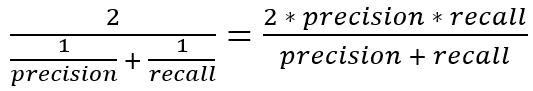
One drawback is that both precision and recall are given equal importance due to which according to our application we may need one higher than the other and F1 score may not be the exact metric for it. Therefore either weighted-F1 score or seeing the PR or ROC curve can help.

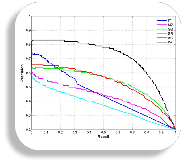
PR curve

It is the curve between precision and recall for various threshold values. In the figure below we have 6 predictors showing their respective precision-recall curve for various threshold values. The top right part of the graph is the ideal space where we get high precision and recall. Based on our application we can choose the predictor and the threshold value. PR AUC is just the area under the curve. The higher its numerical value the better.

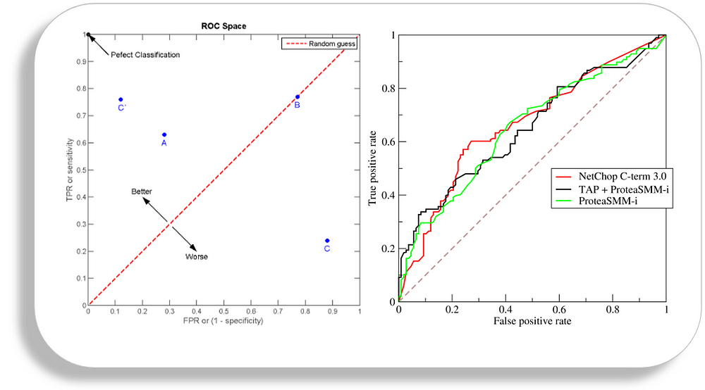
ROC curve

ROC stands for receiver operating characteristic and the graph is plotted against TPR and FPR for various threshold values. As TPR increases FPR also increases. As you can see in the first figure, we have four categories and we want the threshold value that leads us closer to the top left corner. Comparing different predictors (here 3) on a given dataset also becomes easy as you can see in figure 2, one can choose the threshold according to the application at hand. ROC AUC is just the area under the curve, the higher its numerical value the better.

PR vs ROC curve

Both the metrics are widely used to judge a models performance.

Which one to use PR or ROC?

The answer lies in TRUE NEGATIVES.

Due to the absence of TN in the precision-recall equation, they are useful in imbalanced classes. In the case of class imbalance when there is a majority of the negative class. The metric doesn’t take much into consideration the high number of TRUE NEGATIVES of the negative class which is in majority, giving better resistance to the imbalance. This is important when the detection of the positive class is very important.

Like to detect cancer patients, which has a high class imbalance because very few have it out of all the diagnosed. We certainly don’t want to miss on a person having cancer and going undetected (recall) and be sure the detected one is having it (precision).

Due to the consideration of TN or the negative class in the ROC equation, it is useful when both the classes are important to us. Like the detection of cats and dog. The importance of true negatives makes sure that both the classes are given importance, like the output of a CNN model in determining the image is of a cat or a dog.

ROC (Receiver Operating Characteristic) curves and PR (Precision-Recall) curves are both used to evaluate the performance of classification models, particularly in binary classification problems. They visualize the trade-off between different aspects of a model’s predictions, but they focus on different aspects of performance.

ROC Curve:

The ROC curve plots the True Positive Rate (TPR) against the False Positive Rate (FPR) at various threshold settings.
TPR is also known as Recall or Sensitivity. It’s the ratio of correctly predicted positive instances to the total actual positive instances.
FPR is the ratio of incorrectly predicted positive instances to the total actual negative instances.
The ROC curve helps you understand how well your model can distinguish between the two classes across different probability thresholds.
The area under the ROC curve (AUC-ROC) is a common metric used to summarize the overall performance of a model. AUC-ROC provides an aggregate measure of how well the model ranks positive and negative instances.

Precision-Recall Curve:

The PR curve plots Precision against Recall at various threshold settings.
Precision is the ratio of correctly predicted positive instances to the total predicted positive instances.
Recall is the same as TPR, the ratio of correctly predicted positive instances to the total actual positive instances.
The PR curve is particularly useful when dealing with imbalanced datasets, where one class is much more frequent than the other. It focuses on how well the model performs on the positive class.
The area under the PR curve (AUC-PR) is a metric that quantifies the overall performance of the model with respect to precision and recall. AUC-PR gives you an indication of how well the model’s predictions are in terms of positive class identification.

Key Differences:

Focus: ROC curves focus on the trade-off between TPR and FPR, which can be useful when the class distribution is relatively balanced. PR curves, on the other hand, emphasize the trade-off between Precision and Recall, which is particularly important when dealing with imbalanced datasets.
Imbalance: PR curves are more informative when dealing with imbalanced datasets, as they highlight the model’s ability to correctly identify positive instances (higher Recall) while maintaining a low false positive rate (higher Precision).
Interpretation: ROC curves are useful to assess the overall ability of a model to discriminate between classes, regardless of the class distribution. PR curves are more informative about the model’s performance on the positive class.
AUC Interpretation: AUC-ROC and AUC-PR both range between 0 and 1, with higher values indicating better performance. AUC-ROC is more suitable when you’re interested in the general predictive ability of the model across all thresholds, while AUC-PR is better when dealing with imbalanced classes.

In summary, while both ROC and PR curves provide insights into a model’s performance, the choice between them depends on the specific characteristics of your dataset, the class distribution, and the performance aspects you want to focus on.

How to evaluate model’s performance

ByMin Wang

TP, FP, TN, FN

F1 score

PR curve

ROC curve

PR vs ROC curve

By Min Wang

Related Post

Build your own GPU

How to run stable diffusion on CPU boxes

add llama-cpp-python to kubernet cluster

Leave a Reply Cancel reply

You missed

video streaming HLS, DASH

c++ share_ptr pass by value or reference

postfix transport_maps ( routing based on destination domain )

Build your own GPU